Differentiable Image Parameterizations

Neural networks trained to classify images have a remarkable — and surprising! — capacity to generate images. Techniques such as DeepDream , style transfer, and feature visualization leverage this capacity as a powerful tool for exploring the inner workings of neural networks, and to fuel a small artistic movement based on neural art.

All these techniques work in roughly the same way. Neural networks used in computer vision have a rich internal representation of the images they look at. We can use this representation to describe the properties we want an image to have (e.g. style), and then optimize the input image to have those properties. This kind of optimization is possible because the networks are differentiable with respect to their inputs: we can slightly tweak the image to better fit the desired properties, and then iteratively apply such tweaks in gradient descent.

Typically, we parameterize the input image as the RGB values of each pixel, but that isn’t the only way. As long as the mapping from parameters to images is differentiable, we can still optimize alternative parameterizations with gradient descent.

1: As long as an image parameterization is differentiable, we can backpropagate ( ) through it.

Differentiable image parameterizations invite us to ask “what kind of image generation process can we backpropagate through?” The answer is quite a lot, and some of the more exotic possibilities can create a wide range of interesting effects, including 3D neural art, images with transparency, and aligned interpolation. Previous work using specific unusual image parameterizations has shown exciting results — we think that zooming out and looking at this area as a whole suggests there’s even more potential.

Why Does Parameterization Matter?

It may seem surprising that changing the parameterization of an optimization problem can significantly change the result, despite the objective function that is actually being optimized remaining the same. We see four reasons why the choice of parameterization can have a significant effect:

(1) - Improved Optimization - Transforming the input to make an optimization problem easier — a technique called “preconditioning” — is a staple of optimization. Preconditioning is most often presented as a transformation of the gradient (usually multiplying it by a positive definite “preconditioner” matrix). However, this is equivalent to optimizing an alternate parameterization of the input. We find that simple changes in parameterization make image optimization for neural art and image optimization much easier.

(2) - Basins of Attraction - When we optimize the input to a neural network, there are often many different solutions, corresponding to different local minima. Training deep neural networks characterized by complex optimization landscapes , which may have many equally good local minima for a given objective. (Note that finding the global minimum is not always desirable as it may result in an overfitted model .) Thus, it’s probably not surprising that optimizing the input to a neural network would also have many local minima. The probability of our optimization process falling into any particular local minima is controlled by its basin of attraction (i.e., the region of the optimization landscape under the influence of the minimum). Changing the parameterization of an optimization problem is known to change the sizes of different basins of attraction, influencing the likely result.

(3) - Additional Constraints - Some parameterizations cover only a subset of possible inputs, rather than the entire space. An optimizer working in such a parameterization will still find solutions that minimize or maximize the objective function, but they’ll be subject to the constraints of the parameterization. By picking the right set of constraints, one can impose a variety of constraints, ranging from simple constraints (e.g., the boundary of the image must be black), to rich, subtle constraints.

(4) - Implicitly Optimizing other Objects - A parameterization may internally use a different kind of object than the one it outputs and we optimize for. For example, while the natural input to a vision network is an RGB image, we can parameterize that image as a rendering of a 3D object and, by backpropagating through the rendering process, optimize that instead. Because the 3D object has more degrees of freedom than the image, we generally use a stochastic parameterization that produces images rendered from different perspectives.

In the rest of the article we give concrete examples where such approaches are beneficial and lead to surprising and interesting visual results.

Aligned Feature Visualization Interpolation

Feature visualization is most often used to visualize individual neurons, but it can also be used to visualize combinations of neurons, in order to study how they interact . Instead of optimizing an image to make a single neuron fire, one optimizes it to make multiple neurons fire.

When we want to really understand the interaction between two neurons, we can go a step further and create multiple visualizations, gradually shifting the objective from optimizing one neuron to putting more weight on the other neuron firing. This is in some ways similar to interpolation in the latent spaces of generative models like GANs.

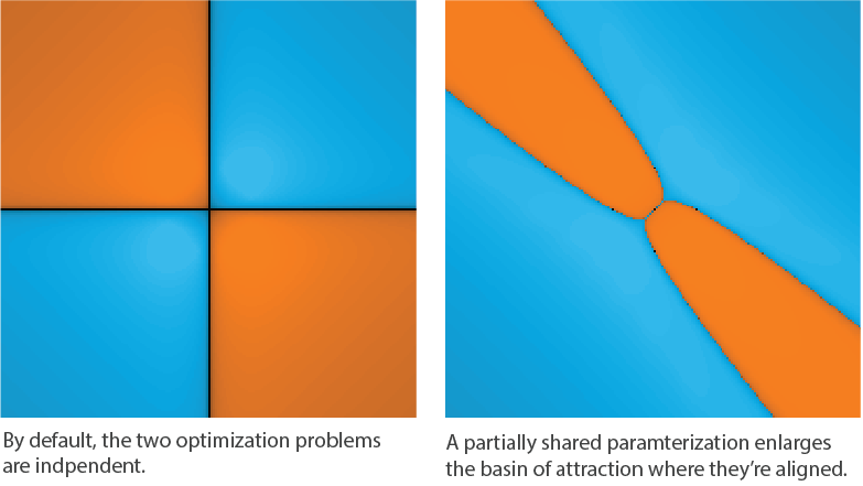
Despite this, there is a small challenge: feature visualization is stochastic. Even if you optimize for the exact same objective, the visualization will be laid out differently each time. Normally, this isn’t a problem, but it does detract from the interpolation visualizations. If we make them naively, the resulting visualizations will be unaligned: visual landmarks such as eyes appear in different locations in each image. This lack of alignment can make it harder to see the difference due to slightly different objectives, because they’re swamped by the much larger differences in layout.

We can see the issue with independent optimization if we look at the interpolated frames as an animation:

How can we achieve this aligned interpolation, where visual landmarks do not move between frames? There are a number of possible approaches one could try For example, one could explicitly penalize differences between adjacent frames. Our final result and our colab notebook use this technique in combination with a shared parameterization. , one of which is using a shared parameterization: each frame is parameterized as a combination of its own unique parameterization, and a single shared one.

By partially sharing a parameterization between frames, we encourage the resulting visualizations to naturally align. Intuitively, the shared parameterization provides a common reference for the displacement of visual landmarks, while the unique one gives to each frame its own visual appeal based on its interpolation weights. Concretely, we combine a usually lower-resolution shared parameterization $P_{\text{shared}}$ and full-resolution independent parameterizations $P_{\text{unique}}^i$ that are unique to each frame $i$ of the visualization. Each individual frame $i$ is then parameterized as a combination $P^i$ of the two, $P^i = \sigma(P_{\text{unique}}^i + P_{\text{shared}})$ , where $\sigma$ is the logistic sigmoid function. This parameterization doesn’t change the objective, but it does enlarge the (2) basins of attraction where the visualizations are aligned. We can explicitly visualize how shared parameterization affects the basins of attraction in a toy example. Let’s consider optimizing two variables $x$ and $y$ to both minimize $L(z)= (z^2-1)^2$ . Since $L(z)$ has two basins of attraction $z=1$ or $z=-1$ , the pair of optimization problems has four solutions: $(x,y) = (1,1)$ , $(x,y) = (-1,1)$ , $(x,y) = (1,-1)$ , or $(x,y) = (-1,-1)$ . Let’s consider randomly initializing $x$ and $y$ , and then optimizing them. Normally, the optimization problems are independent, so $x$ and $y$ are equally likely to come to unaligned solutions (where they have different signs) as aligned ones. But if we add a shared parameterization, the problems become coupled and the basin of attraction where they’re aligned becomes bigger.

This is an initial example of how differentiable parameterizations in general can be a useful additional tool in visualizing neural networks.

Style Transfer with non-VGG architectures

Neural style transfer has a mystery: despite its remarkable success, almost all style transfer is done with variants of the VGG architecture. This isn’t because no one is interested in doing style transfer on other architectures, but because attempts to do it on other architectures consistently work poorly. Examples of experiments performed with different architectures can be found on Medium, Reddit and Twitter.

Several hypotheses have been proposed to explain why VGG works so much better than other models. One suggested explanation is that VGG’s large size causes it to capture information that other models discard. This extra information, the hypothesis goes, isn’t helpful for classification, but it does cause the model to work better for style transfer. An alternate hypothesis is that other models downsample more aggressively than VGG, losing spatial information. We suspect that there may be another factor: most modern vision models have checkerboard artifacts in their gradient , which could make optimization of the stylized image more difficult.

In previous work we found that a decorrelated parameterization can significantly improve optimization. We find the same approach also improves style transfer, allowing us to use a model that did not otherwise produce visually appealing style transfer results:

4: Move the slider under “final image optimization” to compare optimization in pixel space with optimization in a decorrelated space. Both images were created with the same objective and differ only in their parameterization.

Let’s consider this change in a bit more detail. Style transfer involves three images: a content image, a style image, and the image we optimize. All three of these feed into the CNN, and the style transfer objective is based on the differences in how these images activate the CNN. The only change we make is how we parameterize the optimized image. Instead of parameterizing it in terms of pixels (which are highly correlated with their neighbors), we use a scaled Fourier transform.

Our exact implementation can be found in the accompanying notebook. Note that it also uses transformation robustness, which not all implementations of style transfer use.

Compositional Pattern Producing Networks

So far, we’ve explored image parameterizations that are relatively close to how we normally think of images, using pixels or Fourier components. In this section, we explore the possibility of (3) adding additional constraints to the optimization process by using a different parameterization. More specifically, we parameterize our image as a neural network — in particular, a Compositional Pattern Producing Network (CPPN) .

CPPNs are neural networks that map $(x,y)$ positions to image colors:

(x,y) ~\xrightarrow{\tiny CPPN}~ (r,g,b)

By applying the CPPN to a grid of positions, one can make arbitrary resolution images. The parameters of the CPPN network — the weights and biases — determine what image is produced. Depending on the architecture chosen for the CPPN, pixels in the resulting image are constraint to share, up to a certain degree, the color of their neighbors.

Random parameters can produce aesthetically interesting images , but we can produce more interesting images by learning the parameters of the CPPN . Often this is done by evolution ; here we explore the possibility to backpropagate some objective function, such a feature visualization objective. This is easily done since the CPPN network is differentiable as the convolutional neural network and the objective function can be propagated also through the CPPN to update its parameters accordingly. That is to say, CPPNs are a differentiable image parameterization — a general tool for parameterizing images in any neural art or visualization task.

6: CPPNs are a differentiable image parameterization. We can use them for neural art or visualization tasks by backpropagating past the image, through the CPPN to its parameters.

Using CPPNs as image parameterization can add an interesting artistic quality to neural art, vaguely reminiscent of light-paintings.Light-painting is an artistic medium where images are created by manipulating colorful light beams with prisms and mirrors. Notable examples of this technique are the work of Stephen Knapp.

Note that light-painting metaphor here is rather fragile: for example light composition is an additive process, while CPPNs can have negative-weighted connections between layers. At a more theoretical level, they can be seen as constraining the compositional complexity of your images. When used to optimize a feature visualization objective, they produce distinctive images:

7: A Compositional Pattern Producing Network (CPPN) is used as differentiable parameterization for visualizing features at different layers.

The visual quality of the generated images is heavily influenced by the architecture of the chosen CPPN. Not only the shape of the network, i.e., the number of layers and filters, plays a role, but also the chosen activation functions and normalization. For example, deeper networks produce more fine grained details compared to shallow ones. We encourage readers to experiment in generating different images by changing the architecture of the CPPN. This can be easily done by changing the code in the supplementary notebook.

The evolution of the patterns generated by the CPPN are artistic artifacts themselves. To maintain the metaphor of light-paintings, the optimization process correspond to an iterative adjustments of the beam directions and shapes. Because the iterative changes have a more global effect compared to, for example, a pixel parameterization, at the beginning of the optimization only major patterns are visible. By iteratively adjusting the weights, our imaginary beams are positioned in such a way that fine details emerge.

8: Output of CPPNs during training. Control each video by hovering, or tapping it if you are on a mobile device.

By playing with this metaphor, we can also create a new kind of animation that morph one of the above images into a different one. Intuitively, we start from one of the light-paintings and we move the beams to create a different one. This result is in fact achieved by interpolating the weights of the CPPN representations of the two patterns. A number of intermediate frames are then generated by generating an image given the interpolated CPPN representation. As before, changes in the parameter have a global effect and create visually appealing intermediate frames.

9: Interpolating CPPN weights between two learned points.

In this section we presented a parameterization that goes beyond a standard image representation. Neural networks, a CPPN in this case, can be used to parameterize an image that is optimized for a given objective function. More specifically, we combined a feature-visualization objective function with a CPPN parameterization to create infinite-resolution images of distinctive visual style.

Generation of Semi-Transparent Patterns

The neural networks used in this article were trained to receive 2D RGB images as input. Is it possible to use the same network to synthesize artifacts that span (4) beyond this domain? It turns out that we can do so by making our differentiable parameterization define a family of images instead of a single image, and then sampling one or a few images from that family at each optimization step. This is important because many of the objects we’ll explore optimizing have more degrees of freedom than the images going into the network.

To be concrete, let’s consider the case of semi-transparent images. These images have, in addition to the RGB channels, an alpha channel that encodes each pixel’s opacity (in the range $[0,1]$ ). In order to feed such images into a neural network trained on RGB images, we need to somehow collapse the alpha channel. One way to achieve this is to overlay the RGBA image $I$ on top of a background image $BG$ using the standard alpha blending formula In our experiments we use gamma-corrected blending

O_{rgb} ~~=~~ I_{rgb} * I_a ~~+~~ BG_{rgb} * (1 - I_a)

where $I_a$ is the alpha channel of the image $I$ .

If we used a static background $BG$ , such as black, the transparency would merely indicate pixel positions in which that background contributes directly to the optimization objective. In fact, this is equivalent to optimizing an RGB image and making it transparent in areas where its color matches with the background! Intuitively, we’d like transparent areas to correspond to something like “the content of this area could be anything.” Building on this intuition, we use a different random background at every optimization step. We have tried both sampling from real images, and using different types of noise. As long as they were sufficiently randomized, the different distributions did not meaningfully influence the resulting optimization. Thus, for simplicity, we use a smooth 2D gaussian noise.

10: Adding an alpha channel to the image parameterization allows it to represent transparency. Transparent areas are blended with a random background at each step of the optimization.

By default, optimizing our semi-transparent image will make the image fully opaque, so the network can always get its optimal input. To avoid this, we need to change our objective with an objective that encourages some transparency. We find it effective to replace the original objective with:

\text{obj}_{\text{new}} ~~=~~ \text{obj}_{\text{old}} ~~*~~ (1-\text{mean}(I_a))

This new objective automatically balances the original objective $\text{obj}_{\text{old}}$ with reducing the mean transparency. If the image becomes very transparent, it will focus on the original objective. If it becomes too opaque, it will temporarily stop caring about the original objective and focus on decreasing the average opacity.

11: Examples of the optimization of semi transparent images for different layers and units.

It turns out that the generation of semi-transparent images is useful in feature visualization. Feature visualization aims to understand what neurons in a vision model are looking for, by creating images that maximally activate them. Unfortunately, there is no way for these visualizations to distinguish which areas of an image strongly influence a neuron’s activation and those which only marginally do so. This issue does not occur when optimizing for the activation of entire channels, because in that case every pixel has multiple neurons that are close to centered on it. As a consequence, the entire input image gets filled with copies of what those neurons care about strongly.

Ideally, we would like a way for our visualizations to make this distinction in importance — one natural way to represent that a part of the image doesn’t matter is for it to be transparent. Thus, if we optimize an image with an alpha channel and encourage the overall image to be transparent, parts of the image that are unimportant according to the feature visualization objective should become transparent.

Efficient Texture Optimization through 3D Rendering

In the previous section, we were able to use a neural network for RGB images to create a semi-transparent RGBA image. Can we push this even further, creating (4) other kinds of objects even further removed from the RGB input? In this section we explore optimizing 3D objects for a feature-visualization objective. We use a 3D rendering process to turn them into 2D RGB images that can be fed into the network, and backpropagate through the rendering process to optimize the texture of the 3D object.

Our technique is similar to the approach that Athalye et al. used for the creation of real-world adversarial examples, as we rely on the backpropagation of the objective function to randomly sampled views of the 3D model. We differ from existing approaches for artistic texture generation, as we do not modify the geometry of the object during back-propagation. By disentangling the generation of the texture from the position of their vertices, we can create very detailed texture for complex objects.

Before we can describe our approach, we first need to understand how a 3D object is stored and rendered on screen. The object’s geometry is usually saved as a collection of interconnected triangles called triangle mesh or, simply, mesh. To render a realistic model, a texture is painted over the mesh. The texture is saved as an image that is applied to the model by using the so called UV-mapping. Every vertex $c_i$ in the mesh is associated to a $(u_i,v_i)$ coordinate in the texture image. The model is then rendered, i.e. drawn on screen, by coloring every triangle with the region of the image that is delimited by the $(u,v)$ coordinates of its vertices.

A simple naive way to create the 3D object texture would be to optimize an image the normal way and then use it as a texture to paint on the object. However, this approach generates a texture that does not consider the underlying UV-mapping and, therefore, will create a variety of visual artifacts in the rendered object. First, seams are visible on the rendered texture, because the optimization is not aware of the underlying UV-mapping and, therefore, does not optimize the texture consistently along the split patches of the texture. Second, the generated patterns are randomly oriented on different parts of the object (see, e.g., the vertical and wiggly patterns) because they are not consistently oriented in the underlying UV-mapping. Finally generated patterns are inconsistently scaled because the UV-mapping does not enforce a consistent scale between triangle areas and their mapped triangle in the texture.

13: 3D model of the famous Stanford Bunny. You can interact with the model by rotating and zooming. Moreover, you can unfold the object to its two-dimensional texture representation. This unfolding reveals the UV mapping used to store the texture in the texture image. Note how the render-based optimized texture is divided in several patches that allows for a complete and undistorted coverage of the object.

We take a different approach. Instead of directly optimizing the texture, we optimize the texture through renderings of the 3D object, like those the user would eventually see. The following diagram presents an overview of the proposed pipeline:

14: We optimize a texture by backpropagating through the rendering process. This is possible because we know how pixels in the rendered image correspond to pixels in the texture.

We start the process by randomly initializing the texture with a Fourier parameterization. At every training iteration we sample a random camera position, which is oriented towards the center of the bounding box of the object, and we render the textured object as an image. We then backpropagate the gradient of the desired objective function, i.e., the feature of interest in the neural network, to the rendered image.

However, an update of the rendered image does not correspond to an update to the texture that we aim at optimizing. Hence, we need to further propagate the changes to the object’s texture. The propagation is easily implemented by applying a reverse UV-mapping, as for each pixel on screen we know its coordinate in the texture. By modifying the texture, during the following optimization iterations, the rendered image will incorporate the changes applied in the previous iterations.

15: Textures are generated by optimizing for a feature visualization objective function. Seams in the textures are hardly visible and the patterns are correctly oriented.

The resulting textures are consistently optimized along the cuts, hence removing the seams and enforcing an uniform orientation for the rendered object. Morever, since the function optimization is disentangled by the geometry of the object, the resolution of the texture can be arbitrary high. In the next section we will se how this framework can be reused for performing an artistic style transfer to the object’s texture.

Style Transfer for Textures through 3D Rendering

Now that we have established a framework for efficient backpropagation into the UV-mapped texture, we can use it to adapt existing style transfer techniques for 3D objects. Similarly to the 2D case, we aim at redrawing the original object’s texture with the style of a user-provided image. The following diagram presents an overview of the approach:

The algorithm works in similar way to the one presented in the previous section, starting from a randomly initialized texture. At each iteration, we sample a random view point oriented toward the center of the bounding box of the object and we render two images of it: one with the original texture, the content image, and one with the texture that we are currently optimizing, the learned image.

After the content image and learned image are rendered, we optimize for the style-transfer objective function introduced by Gatys et al. and we map the parameterization back in the UV-mapped texture as introduced in the previous section. The procedure is then iterated until the desired blend of content and style is obtained in the target texture.

17: Style Transfer onto various 3D models. Note that visual landmarks in the content texture, such as eyes, show up correctly in the generated texture.

Because every view is optimized independently, the optimization is forced to try to add all the style’s elements at every iteration. For example, if we use as style image the Van Gogh’s “Starry Night” painting, stars will be added in every single view. We found we obtain more pleasing results, such as those presented above, by introducing a sort of “memory” of the style of previous views. To this end, we maintain moving averages of style-representing Gram matrices over the recently sampled viewpoints. On each optimization iteration we compute the style loss against those averaged matrices, instead of the ones computed for that particular view. We use TensorFlow’s tf.stop_gradient method to substitute current Gram matrices with their moving averages on forward pass, while still propagating the correct gradients to the current Gram matrices.

An alternative approach, such as the one employed by , would require sampling multiple viewpoints of the scene at each step, increasing memory requirements. In contrast, our substitution trick can be also used to apply style transfer to high resolution (>10M pixels) images on a single consumer-grade GPU.

The resulting textures combine elements of the desired style, while preserving the characteristics of the original texture. Take as an example the model created by imposing Van Gogh’s starry night as style image. The resulting texture contains the rythmic and vigorous brush strokes that characterize Van Gogh’s work. However, despite the style image’s primarily cold tones, the resulting fur has a warm orange undertone as it is preserved from the original texture. Even more interesting is how the eyes of the bunny are preserved when different styles are transfered. For example, when the style is obtained from the Van Gogh’s painting, the eyes are transformed in a star-like swirl, while if Kandinsky’s work is used, they become abstract patterns that still resemble the original eyes.

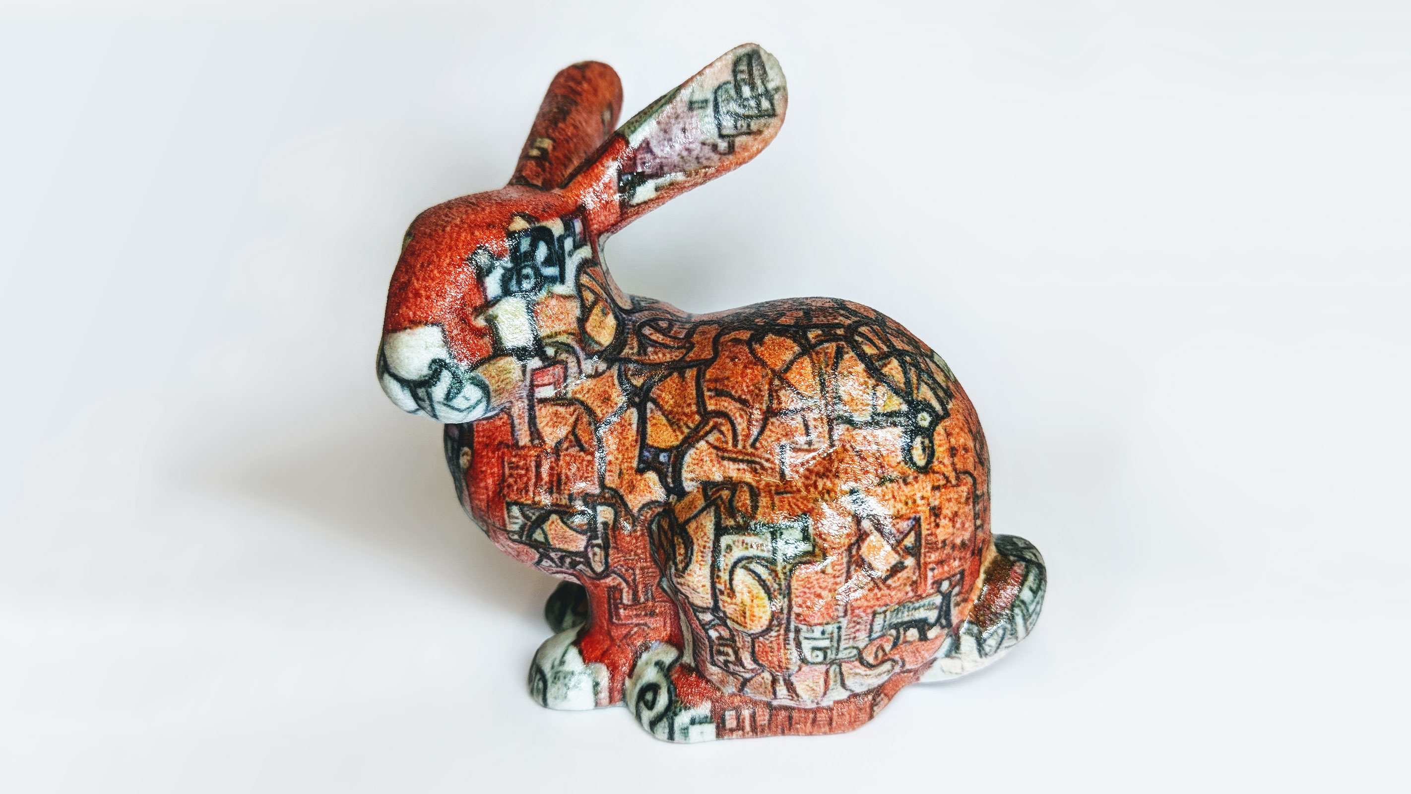
18: 3D print of a style transfer of ”La grand parade sur fond rouge″ (Fernand Leger, 1953) onto the ”Stanford Bunny″ by Greg Turk & Marc Levoy.

Textured models produced with the presented method can be easily used with popular 3D modeling software or game engines. To show this, we 3D printed one of the designs as a real-world physical artifact We used the Full-color Sandstone material..

Conclusions

For the creative artist or researcher, there’s a large space of ways to parameterize images for optimization. This opens up not only dramatically different image results, but also animations and 3D objects! We think the possibilities explored in this article only scratch the surface. For example, one could explore extending the optimization of 3D object textures to optimizing the material or reflectance — or even go the direction of Kato et al. and optimize the mesh vertex positions.

This article focused on differentiable image parameterizations, because they are easy to optimize and cover a wide range of possible applications. But it’s certainly possible to optimize image parameterizations that aren’t differentiable, or are only partly differentiable, using reinforcement learning or evolutionary strategies . Using non-differentiable parameterizations could open up exciting possibilities for image or scene generation.

Additional Resources

Code: tensorflow/lucid
Open-source implementation of our techniques on GitHub

Notebooks:
Direct links to ipynb notebooks corresponding to the respective sections of this paper.

Further Notebooks:
Direct links to ipynb notebooks generally related to topics of this paper, or exploring more technical aspects of the techniques described in this paper.

Experiments on different backgrounds shows additional experiments from Parameterization with Transparency. Amongst other techniques, contains allied and adversarial backgrounds.
Additional Notebook 2

Acknowledgments

We are very grateful to Justin Gilmer, Shan Carter, Dominik Roblek and Amit Patel. Justin generously stepped in to handle the review process of this article. Shan was available for outstanding design insight and implementation advice. Dominik Roblek made the 3D printed example possible, while Amit Patel hunted down an obscure bug in our Style Transfer diagram.

We appreciate the reviewers who put in the time to write in-depth reviews, which helped us improve our paper significantly: Pang Wei Koh, as well as Anonymous Reviewer 2 and Anonymous Reviewer 3. We also thank Matt Sharifi, Arvind Satyanarayan, Ian Johnson, and Vincent Sitzmann for their thoughts, comments, discussions and support.

Lastly, this work was made possible by many open source tools, for which we are grateful. In particular, all of our experiments were based on Tensorflow, most of our interactive diagrams are built in Svelte, and all 3D diagrams use ThreeJS.

Author Contributions

Research: Alex developed the use of transparency, CPPN parameterization, 3D parameterization, and non-VGG style transfer. Chris developed the use of joint parameterization for alignment, and was lightly involved in the development of transparency and 3D models. The final versions presented in the article were refined by Nicola and Ludwig.

Writing & Diagrams: The text was initially drafted by Nicola and refined by the other authors. The interactive diagrams were designed by Ludwig and Nicola. The final notebooks were primarily created by Ludwig, based on earlier code and notebooks by Alex and Chris.

Discussion and Review

Review 1 - Pang Wei Koh
Review 2 - Anonymous
Review 3 - Anonymous

References

Inceptionism: Going deeper into neural networks [HTML]
Mordvintsev, A., Olah, C. and Tyka, M., 2015. Google Research Blog. Retrieved June, Vol 20(14), pp. 5.
A Neural Algorithm of Artistic Style [PDF]
Gatys, L.A., Ecker, A.S. and Bethge, M., 2015. CoRR, Vol abs/1508.06576.
Feature Visualization [link]
Olah, C., Mordvintsev, A. and Schubert, L., 2017. Distill. DOI: 10.23915/distill.00007
Deep neural networks are easily fooled: High confidence predictions for unrecognizable images [PDF]
Nguyen, A.M., Yosinski, J. and Clune, J., 2015. IEEE Conference on Computer Vision and Pattern Recognition, CVPR 2015, Boston, MA, USA, June 7-12, 2015, pp. 427--436.
Synthesizing robust adversarial examples [PDF]
Athalye, A., Engstrom, L., Ilyas, A. and Kwok, K., 2017. arXiv preprint arXiv:1707.07397.
The loss surfaces of multilayer networks [PDF]
Choromanska, A., Henaff, M., Mathieu, M., Arous, G.B. and LeCun, Y., 2015. Artificial Intelligence and Statistics, pp. 192--204.
Very deep convolutional networks for large-scale image recognition [PDF]
Simonyan, K. and Zisserman, A., 2014. arXiv preprint arXiv:1409.1556.
Deconvolution and checkerboard artifacts [link]
Odena, A., Dumoulin, V. and Olah, C., 2016. Distill, Vol 1(10), pp. e3. DOI: 10.23915/distill.00003
Deep Image Prior [PDF]
Ulyanov, D., Vedaldi, A. and Lempitsky, V.S., 2017. CoRR, Vol abs/1711.10925.
Compositional pattern producing networks: A novel abstraction of development [PDF]
Stanley, K.O., 2007. Genetic programming and evolvable machines, Vol 8(2), pp. 131--162. Springer.
Neural Network Generative Art in Javascript [link]
Ha, D., 2015.
Image Regression [HTML]
Karpathy, A., 2014.
Generating Large Images from Latent Vectors [link]
Ha, D., 2016.
Artificial Evolution for Computer Graphics [HTML]
Sims, K., 1991. SIGGRAPH Comput. Graph., Vol 25(4), pp. 319--328. ACM. DOI: 10.1145/127719.122752
Neural 3D Mesh Renderer [PDF]
Kato, H., Ushiku, Y. and Harada, T., 2017. arXiv preprint arXiv:1711.07566.
The Stanford Bunny [link]
Turk, G. and Levoy, M., 2005. Stanford University Computer Graphics Laboratory.
Natural evolution strategies. [PDF]
Wierstra, D., Schaul, T., Glasmachers, T., Sun, Y., Peters, J. and Schmidhuber, J., 2014. Journal of Machine Learning Research, Vol 15(1), pp. 949--980.
Evolution strategies as a scalable alternative to reinforcement learning [link]
Salimans, T., Ho, J., Chen, X. and Sutskever, I., 2017. arXiv preprint arXiv:1703.03864.
Tensorflow: Large-scale machine learning on heterogeneous distributed systems [PDF]
Abadi, M., Agarwal, A., Barham, P., Brevdo, E., Chen, Z., Citro, C., Corrado, G.S., Davis, A., Dean, J., Devin, M., Ghemawat, S., Goodfellow, I.J., Harp, A., Irving, G., Isard, M., Jia, Y., J{\'{o}}zefowicz, R., Kaiser, L., Kudlur, M., Levenberg, J., Man{\'{e}}, D., Monga, R., Moore, S., Murray, D.G., Olah, C., Schuster, M., Shlens, J., Steiner, B., Sutskever, I., Talwar, K., Tucker, P.A., Vanhoucke, V., Vasudevan, V., Vi{\'{e}}gas, F.B., Vinyals, O., Warden, P., Wattenberg, M., Wicke, M., Yu, Y. and Zheng, X., 2016. arXiv preprint arXiv:1603.04467.

Updates and Corrections

If you see mistakes or want to suggest changes, please create an issue on GitHub.

Reuse

Diagrams and text are licensed under Creative Commons Attribution CC-BY 4.0 with the source available on GitHub, unless noted otherwise. The figures that have been reused from other sources don’t fall under this license and can be recognized by a note in their caption: “Figure from …”.

Citation

For attribution in academic contexts, please cite this work as

Mordvintsev, et al., "Differentiable Image Parameterizations", Distill, 2018.

BibTeX citation

@article{mordvintsev2018differentiable,
  author = {Mordvintsev, Alexander and Pezzotti, Nicola and Schubert, Ludwig and Olah, Chris},
  title = {Differentiable Image Parameterizations},
  journal = {Distill},
  year = {2018},
  note = {https://distill.pub/2018/differentiable-parameterizations},
  doi = {10.23915/distill.00012}
}

[mordvintsev2015inceptionism] Inceptionism: Going deeper into neural networks [HTML]
Mordvintsev, A., Olah, C. and Tyka, M., 2015. Google Research Blog. Retrieved June, Vol 20(14), pp. 5.

[gatys2015] A Neural Algorithm of Artistic Style [PDF]
Gatys, L.A., Ecker, A.S. and Bethge, M., 2015. CoRR, Vol abs/1508.06576.

[olah2017feature] Feature Visualization [link]
Olah, C., Mordvintsev, A. and Schubert, L., 2017. Distill. DOI: 10.23915/distill.00007

[Nguyen2015:easilyFooled] Deep neural networks are easily fooled: High confidence predictions for unrecognizable images [PDF]
Nguyen, A.M., Yosinski, J. and Clune, J., 2015. IEEE Conference on Computer Vision and Pattern Recognition, CVPR 2015, Boston, MA, USA, June 7-12, 2015, pp. 427--436.

[athalye2017synthesizing] Synthesizing robust adversarial examples [PDF]
Athalye, A., Engstrom, L., Ilyas, A. and Kwok, K., 2017. arXiv preprint arXiv:1707.07397.

[choromanska2015loss] The loss surfaces of multilayer networks [PDF]
Choromanska, A., Henaff, M., Mathieu, M., Arous, G.B. and LeCun, Y., 2015. Artificial Intelligence and Statistics, pp. 192--204.

[simonyan2014vgg] Very deep convolutional networks for large-scale image recognition [PDF]
Simonyan, K. and Zisserman, A., 2014. arXiv preprint arXiv:1409.1556.

[odena2016deconvolution] Deconvolution and checkerboard artifacts [link]
Odena, A., Dumoulin, V. and Olah, C., 2016. Distill, Vol 1(10), pp. e3. DOI: 10.23915/distill.00003

[ulyanov2017deepimageprior] Deep Image Prior [PDF]
Ulyanov, D., Vedaldi, A. and Lempitsky, V.S., 2017. CoRR, Vol abs/1711.10925.

[stanley2007cppn] Compositional pattern producing networks: A novel abstraction of development [PDF]
Stanley, K.O., 2007. Genetic programming and evolvable machines, Vol 8(2), pp. 131--162. Springer.

[CPPN:random] Neural Network Generative Art in Javascript [link]
Ha, D., 2015.

[karpathy2014cppns] Image Regression [HTML]
Karpathy, A., 2014.

[ha2016cppns] Generating Large Images from Latent Vectors [link]
Ha, D., 2016.

[sims1991evolution] Artificial Evolution for Computer Graphics [HTML]
Sims, K., 1991. SIGGRAPH Comput. Graph., Vol 25(4), pp. 319--328. ACM. DOI: 10.1145/127719.122752

[kato2017neural3D] Neural 3D Mesh Renderer [PDF]
Kato, H., Ushiku, Y. and Harada, T., 2017. arXiv preprint arXiv:1711.07566.

[turk2005stanfordBunny] The Stanford Bunny [link]
Turk, G. and Levoy, M., 2005. Stanford University Computer Graphics Laboratory.

[wierstra2014naturalEvolutionStrategies] Natural evolution strategies. [PDF]
Wierstra, D., Schaul, T., Glasmachers, T., Sun, Y., Peters, J. and Schmidhuber, J., 2014. Journal of Machine Learning Research, Vol 15(1), pp. 949--980.

[salimans2017evolution] Evolution strategies as a scalable alternative to reinforcement learning [link]
Salimans, T., Ho, J., Chen, X. and Sutskever, I., 2017. arXiv preprint arXiv:1703.03864.

[abadi2016tensorflow] Tensorflow: Large-scale machine learning on heterogeneous distributed systems [PDF]
Abadi, M., Agarwal, A., Barham, P., Brevdo, E., Chen, Z., Citro, C., Corrado, G.S., Davis, A., Dean, J., Devin, M., Ghemawat, S., Goodfellow, I.J., Harp, A., Irving, G., Isard, M., Jia, Y., J{\'{o}}zefowicz, R., Kaiser, L., Kudlur, M., Levenberg, J., Man{\'{e}}, D., Monga, R., Moore, S., Murray, D.G., Olah, C., Schuster, M., Shlens, J., Steiner, B., Sutskever, I., Talwar, K., Tucker, P.A., Vanhoucke, V., Vasudevan, V., Vi{\'{e}}gas, F.B., Vinyals, O., Warden, P., Wattenberg, M., Wicke, M., Yu, Y. and Zheng, X., 2016. arXiv preprint arXiv:1603.04467.