This article is one of two Distill publications about graph neural networks. Take a look at Understanding Convolutions on Graphs
Graphs are all around us; real world objects are often defined in terms of their connections to other things. A set of objects, and the connections between them, are naturally expressed as a graph. Researchers have developed neural networks that operate on graph data (called graph neural networks, or GNNs) for over a decade
This article explores and explains modern graph neural networks. We divide this work into four parts. First, we look at what kind of data is most naturally phrased as a graph, and some common examples. Second, we explore what makes graphs different from other types of data, and some of the specialized choices we have to make when using graphs. Third, we build a modern GNN, walking through each of the parts of the model, starting with historic modeling innovations in the field. We move gradually from a bare-bones implementation to a state-of-the-art GNN model. Fourth and finally, we provide a GNN playground where you can play around with a real-word task and dataset to build a stronger intuition of how each component of a GNN model contributes to the predictions it makes.
To start, let’s establish what a graph is. A graph represents the relations (edges) between a collection of entities (nodes).
To further describe each node, edge or the entire graph, we can store information in each of these pieces of the graph.
We can additionally specialize graphs by associating directionality to edges (directed, undirected).

Graphs are very flexible data structures, and if this seems abstract now, we will make it concrete with examples in the next section.
Graphs and where to find them
You’re probably already familiar with some types of graph data, such as social networks. However, graphs are an extremely powerful and general representation of data, we will show two types of data that you might not think could be modeled as graphs: images and text. Although counterintuitive, one can learn more about the symmetries and structure of images and text by viewing them as graphs,, and build an intuition that will help understand other less grid-like graph data, which we will discuss later.
Images as graphs
We typically think of images as rectangular grids with image channels, representing them as arrays (e.g., 244x244x3 floats). Another way to think of images is as graphs with regular structure, where each pixel represents a node and is connected via an edge to adjacent pixels. Each non-border pixel has exactly 8 neighbors, and the information stored at each node is a 3-dimensional vector representing the RGB value of the pixel.
A way of visualizing the connectivity of a graph is through its adjacency matrix. We order the nodes, in this case each of 25 pixels in a simple 5x5 image of a smiley face, and fill a matrix of $n_{nodes} \times n_{nodes}$ with an entry if two nodes share an edge. Note that each of these three representations below are different views of the same piece of data.
Text as graphs
We can digitize text by associating indices to each character, word, or token, and representing text as a sequence of these indices. This creates a simple directed graph, where each character or index is a node and is connected via an edge to the node that follows it.
Of course, in practice, this is not usually how text and images are encoded: these graph representations are redundant since all images and all text will have very regular structures. For instance, images have a banded structure in their adjacency matrix because all nodes (pixels) are connected in a grid. The adjacency matrix for text is just a diagonal line, because each word only connects to the prior word, and to the next one.
Graph-valued data in the wild
Graphs are a useful tool to describe data you might already be familiar with. Let’s move on to data which is more heterogeneously structured. In these examples, the number of neighbors to each node is variable (as opposed to the fixed neighborhood size of images and text). This data is hard to phrase in any other way besides a graph.
Molecules as graphs. Molecules are the building blocks of matter, and are built of atoms and electrons in 3D space. All particles are interacting, but when a pair of atoms are stuck in a stable distance from each other, we say they share a covalent bond. Different pairs of atoms and bonds have different distances (e.g. single-bonds, double-bonds). It’s a very convenient and common abstraction to describe this 3D object as a graph, where nodes are atoms and edges are covalent bonds.
Social networks as graphs. Social networks are tools to study patterns in collective behaviour of people, institutions and organizations. We can build a graph representing groups of people by modelling individuals as nodes, and their relationships as edges.
Unlike image and text data, social networks do not have identical adjacency matrices.
Citation networks as graphs. Scientists routinely cite other scientists’ work when publishing papers. We can visualize these networks of citations as a graph, where each paper is a node, and each directed edge is a citation between one paper and another. Additionally, we can add information about each paper into each node, such as a word embedding of the abstract. (see
Other examples. In computer vision, we sometimes want to tag objects in visual scenes. We can then build graphs by treating these objects as nodes, and their relationships as edges. Machine learning models, programming code
The structure of real-world graphs can vary greatly between different types of data — some graphs have many nodes with few connections between them, or vice versa. Graph datasets can vary widely (both within a given dataset, and between datasets) in terms of the number of nodes, edges, and the connectivity of nodes.
Summary statistics on graphs found in the real world. Numbers are dependent on featurization decisions. More useful statistics and graphs can be found in KONECT
What types of problems have graph structured data?
We have described some examples of graphs in the wild, but what tasks do we want to perform on this data? There are three general types of prediction tasks on graphs: graph-level, node-level, and edge-level.
In a graph-level task, we predict a single property for a whole graph. For a node-level task, we predict some property for each node in a graph. For an edge-level task, we want to predict the property or presence of edges in a graph.
For the three levels of prediction problems described above (graph-level, node-level, and edge-level), we will show that all of the following problems can be solved with a single model class, the GNN. But first, let’s take a tour through the three classes of graph prediction problems in more detail, and provide concrete examples of each.
Graph-level task
In a graph-level task, our goal is to predict the property of an entire graph. For example, for a molecule represented as a graph, we might want to predict what the molecule smells like, or whether it will bind to a receptor implicated in a disease.
This is analogous to image classification problems with MNIST and CIFAR, where we want to associate a label to an entire image. With text, a similar problem is sentiment analysis where we want to identify the mood or emotion of an entire sentence at once.
Node-level task
Node-level tasks are concerned with predicting the identity or role of each node within a graph.
A classic example of a node-level prediction problem is Zach’s karate club.
Following the image analogy, node-level prediction problems are analogous to image segmentation, where we are trying to label the role of each pixel in an image. With text, a similar task would be predicting the parts-of-speech of each word in a sentence (e.g. noun, verb, adverb, etc).
Edge-level task
The remaining prediction problem in graphs is edge prediction.
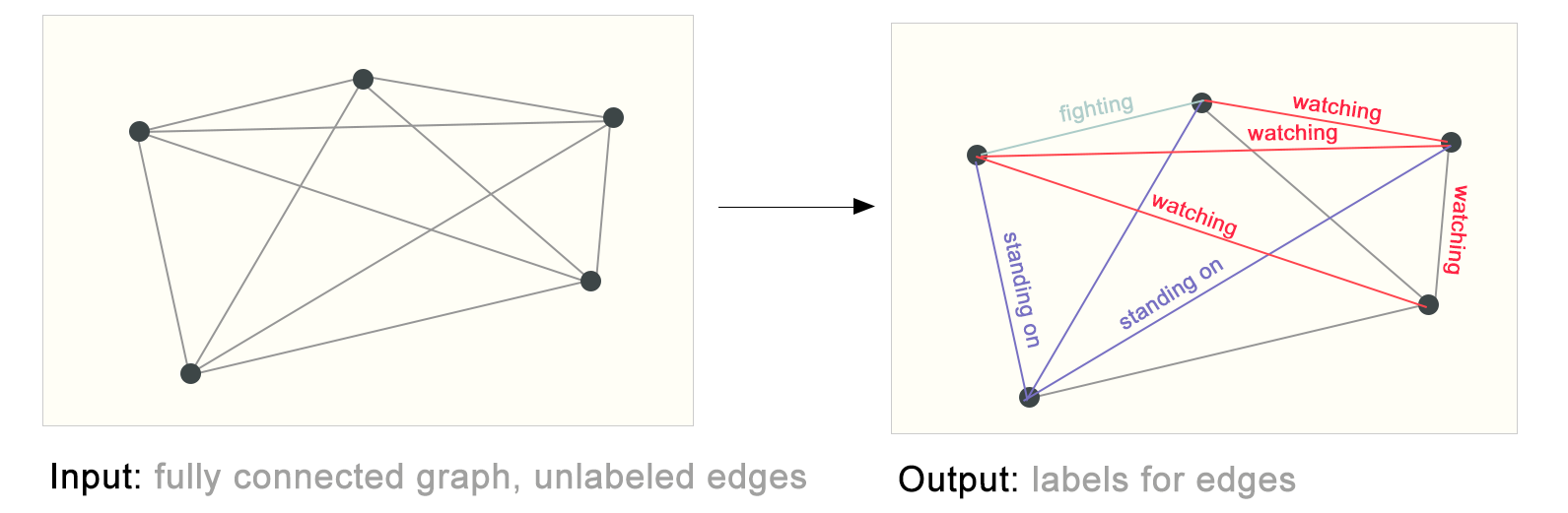
One example of edge-level inference is in image scene understanding. Beyond identifying objects in an image, deep learning models can be used to predict the relationship between them. We can phrase this as an edge-level classification: given nodes that represent the objects in the image, we wish to predict which of these nodes share an edge or what the value of that edge is. If we wish to discover connections between entities, we could consider the graph fully connected and based on their predicted value prune edges to arrive at a sparse graph.

The challenges of using graphs in machine learning
So, how do we go about solving these different graph tasks with neural networks? The first step is to think about how we will represent graphs to be compatible with neural networks.
Machine learning models typically take rectangular or grid-like arrays as input. So, it’s not immediately intuitive how to represent them in a format that is compatible with deep learning. Graphs have up to four types of information that we will potentially want to use to make predictions: nodes, edges, global-context and connectivity. The first three are relatively straightforward: for example, with nodes we can form a node feature matrix $N$ by assigning each node an index $i$ and storing the feature for $node_i$ in $N$. While these matrices have a variable number of examples, they can be processed without any special techniques.
However, representing a graph’s connectivity is more complicated. Perhaps the most obvious choice would be to use an adjacency matrix, since this is easily tensorisable. However, this representation has a few drawbacks. From the example dataset table, we see the number of nodes in a graph can be on the order of millions, and the number of edges per node can be highly variable. Often, this leads to very sparse adjacency matrices, which are space-inefficient.
Another problem is that there are many adjacency matrices that can encode the same connectivity, and there is no guarantee that these different matrices would produce the same result in a deep neural network (that is to say, they are not permutation invariant).
For example, the Othello graph from before can be described equivalently with these two adjacency matrices. It can also be described with every other possible permutation of the nodes.


The example below shows every adjacency matrix that can describe this small graph of 4 nodes. This is already a significant number of adjacency matrices–for larger examples like Othello, the number is untenable.
One elegant and memory-efficient way of representing sparse matrices is as adjacency lists. These describe the connectivity of edge $e_k$ between nodes $n_i$ and $n_j$ as a tuple (i,j) in the k-th entry of an adjacency list. Since we expect the number of edges to be much lower than the number of entries for an adjacency matrix ($n_{nodes}^2$), we avoid computation and storage on the disconnected parts of the graph.
To make this notion concrete, we can see how information in different graphs might be represented under this specification:
It should be noted that the figure uses scalar values per node/edge/global, but most practical tensor representations have vectors per graph attribute. Instead of a node tensor of size $[n_{nodes}]$ we will be dealing with node tensors of size $[n_{nodes}, node_{dim}]$. Same for the other graph attributes.
Graph Neural Networks
Now that the graph’s description is in a matrix format that is permutation invariant, we will describe using graph neural networks (GNNs) to solve graph prediction tasks. A GNN is an optimizable transformation on all attributes of the graph (nodes, edges, global-context) that preserves graph symmetries (permutation invariances). We’re going to build GNNs using the “message passing neural network” framework proposed by Gilmer et al.
The simplest GNN
With the numerical representation of graphs that we’ve constructed above (with vectors instead of scalars), we are now ready to build a GNN. We will start with the simplest GNN architecture, one where we learn new embeddings for all graph attributes (nodes, edges, global), but where we do not yet use the connectivity of the graph.
This GNN uses a separate multilayer perceptron (MLP) (or your favorite differentiable model) on each component of a graph; we call this a GNN layer. For each node vector, we apply the MLP and get back a learned node-vector. We do the same for each edge, learning a per-edge embedding, and also for the global-context vector, learning a single embedding for the entire graph.

As is common with neural networks modules or layers, we can stack these GNN layers together.
Because a GNN does not update the connectivity of the input graph, we can describe the output graph of a GNN with the same adjacency list and the same number of feature vectors as the input graph. But, the output graph has updated embeddings, since the GNN has updated each of the node, edge and global-context representations.
GNN Predictions by Pooling Information
We have built a simple GNN, but how do we make predictions in any of the tasks we described above?
We will consider the case of binary classification, but this framework can easily be extended to the multi-class or regression case. If the task is to make binary predictions on nodes, and the graph already contains node information, the approach is straightforward — for each node embedding, apply a linear classifier.

However, it is not always so simple. For instance, you might have information in the graph stored in edges, but no information in nodes, but still need to make predictions on nodes. We need a way to collect information from edges and give them to nodes for prediction. We can do this by pooling. Pooling proceeds in two steps:
For each item to be pooled, gather each of their embeddings and concatenate them into a matrix.
The gathered embeddings are then aggregated, usually via a sum operation.
We represent the pooling operation by the letter $\rho$, and denote that we are gathering information from edges to nodes as $p_{E_n \to V_{n}}$.
So If we only have edge-level features, and are trying to predict binary node information, we can use pooling to route (or pass) information to where it needs to go. The model looks like this.

If we only have node-level features, and are trying to predict binary edge-level information, the model looks like this.

If we only have node-level features, and need to predict a binary global property, we need to gather all available node information together and aggregate them. This is similar to Global Average Pooling layers in CNNs. The same can be done for edges.

In our examples, the classification model $c$ can easily be replaced with any differentiable model, or adapted to multi-class classification using a generalized linear model.

Now we’ve demonstrated that we can build a simple GNN model, and make binary predictions by routing information between different parts of the graph. This pooling technique will serve as a building block for constructing more sophisticated GNN models. If we have new graph attributes, we just have to define how to pass information from one attribute to another.
Note that in this simplest GNN formulation, we’re not using the connectivity of the graph at all inside the GNN layer. Each node is processed independently, as is each edge, as well as the global context. We only use connectivity when pooling information for prediction.
Passing messages between parts of the graph
We could make more sophisticated predictions by using pooling within the GNN layer, in order to make our learned embeddings aware of graph connectivity. We can do this using message passing
Message passing works in three steps:
For each node in the graph, gather all the neighboring node embeddings (or messages), which is the $g$ function described above.
Aggregate all messages via an aggregate function (like sum).
All pooled messages are passed through an update function, usually a learned neural network.
Just as pooling can be applied to either nodes or edges, message passing can occur between either nodes or edges.
These steps are key for leveraging the connectivity of graphs. We will build more elaborate variants of message passing in GNN layers that yield GNN models of increasing expressiveness and power.
This sequence of operations, when applied once, is the simplest type of message-passing GNN layer.
This is reminiscent of standard convolution: in essence, message passing and convolution are operations to aggregate and process the information of an element’s neighbors in order to update the element’s value. In graphs, the element is a node, and in images, the element is a pixel. However, the number of neighboring nodes in a graph can be variable, unlike in an image where each pixel has a set number of neighboring elements.
By stacking message passing GNN layers together, a node can eventually incorporate information from across the entire graph: after three layers, a node has information about the nodes three steps away from it.
We can update our architecture diagram to include this new source of information for nodes:

Learning edge representations
Our dataset does not always contain all types of information (node, edge, and global context). When we want to make a prediction on nodes, but our dataset only has edge information, we showed above how to use pooling to route information from edges to nodes, but only at the final prediction step of the model. We can share information between nodes and edges within the GNN layer using message passing.
We can incorporate the information from neighboring edges in the same way we used neighboring node information earlier, by first pooling the edge information, transforming it with an update function, and storing it.
However, the node and edge information stored in a graph are not necessarily the same size or shape, so it is not immediately clear how to combine them. One way is to learn a linear mapping from the space of edges to the space of nodes, and vice versa. Alternatively, one may concatenate them together before the update function.

Which graph attributes we update and in which order we update them is one design decision when constructing GNNs. We could choose whether to update node embeddings before edge embeddings, or the other way around. This is an open area of research with a variety of solutions– for example we could update in a ‘weave’ fashion

Adding global representations
There is one flaw with the networks we have described so far: nodes that are far away from each other in the graph may never be able to efficiently transfer information to one another, even if we apply message passing several times. For one node, If we have k-layers, information will propagate at most k-steps away. This can be a problem for situations where the prediction task depends on nodes, or groups of nodes, that are far apart. One solution would be to have all nodes be able to pass information to each other.
Unfortunately for large graphs, this quickly becomes computationally expensive (although this approach, called ‘virtual edges’, has been used for small graphs such as molecules).
One solution to this problem is by using the global representation of a graph (U) which is sometimes called a master node

In this view all graph attributes have learned representations, so we can leverage them during pooling by conditioning the information of our attribute of interest with respect to the rest. For example, for one node we can consider information from neighboring nodes, connected edges and the global information. To condition the new node embedding on all these possible sources of information, we can simply concatenate them. Additionally we may also map them to the same space via a linear map and add them or apply a feature-wise modulation layer

GNN playground
We’ve described a wide range of GNN components here, but how do they actually differ in practice? This GNN playground allows you to see how these different components and architectures contribute to a GNN’s ability to learn a real task.
Our playground shows a graph-level prediction task with small molecular graphs. We use the the Leffingwell Odor Dataset
To simplify the problem, we consider only a single binary label per molecule, classifying if a molecular graph smells “pungent” or not, as labeled by a professional perfumer. We say a molecule has a “pungent” scent if it has a strong, striking smell. For example, garlic and mustard, which might contain the molecule allyl alcohol have this quality. The molecule piperitone, often used for peppermint-flavored candy, is also described as having a pungent smell.
We represent each molecule as a graph, where atoms are nodes containing a one-hot encoding for its atomic identity (Carbon, Nitrogen, Oxygen, Fluorine) and bonds are edges containing a one-hot encoding its bond type (single, double, triple or aromatic).
Our general modeling template for this problem will be built up using sequential GNN layers, followed by a linear model with a sigmoid activation for classification. The design space for our GNN has many levers that can customize the model:
The number of GNN layers, also called the depth.
The dimensionality of each attribute when updated. The update function is a 1-layer MLP with a relu activation function and a layer norm for normalization of activations.
The aggregation function used in pooling: max, mean or sum.
The graph attributes that get updated, or styles of message passing: nodes, edges and global representation. We control these via boolean toggles (on or off). A baseline model would be a graph-independent GNN (all message-passing off) which aggregates all data at the end into a single global attribute. Toggling on all message-passing functions yields a GraphNets architecture.
To better understand how a GNN is learning a task-optimized representation of a graph, we also look at the penultimate layer activations of the GNN. These ‘graph embeddings’ are the outputs of the GNN model right before prediction. Since we are using a generalized linear model for prediction, a linear mapping is enough to allow us to see how we are learning representations around the decision boundary.
Since these are high dimensional vectors, we reduce them to 2D via principal component analysis (PCA). A perfect model would visibility separate labeled data, but since we are reducing dimensionality and also have imperfect models, this boundary might be harder to see.
Play around with different model architectures to build your intuition. For example, see if you can edit the molecule on the left to make the model prediction increase. Do the same edits have the same effects for different model architectures?
Some empirical GNN design lessons
When exploring the architecture choices above, you might have found some models have better performance than others. Are there some clear GNN design choices that will give us better performance? For example, do deeper GNN models perform better than shallower ones? or is there a clear choice between aggregation functions? The answers are going to depend on the data,
With the following interactive figure, we explore the space of GNN architectures and the performance of this task across a few major design choices: Style of message passing, the dimensionality of embeddings, number of layers, and aggregation operation type.
Each point in the scatter plot represents a model: the x axis is the number of trainable variables, and the y axis is the performance. Hover over a point to see the GNN architecture parameters.
The first thing to notice is that, surprisingly, a higher number of parameters does correlate with higher performance. GNNs are a very parameter-efficient model type: for even a small number of parameters (3k) we can already find models with high performance.
Next, we can look at the distributions of performance aggregated based on the dimensionality of the learned representations for different graph attributes.
We can notice that models with higher dimensionality tend to have better mean and lower bound performance but the same trend is not found for the maximum. Some of the top-performing models can be found for smaller dimensions. Since higher dimensionality is going to also involve a higher number of parameters, these observations go in hand with the previous figure.
Next we can see the breakdown of performance based on the number of GNN layers.
The box plot shows a similar trend, while the mean performance tends to increase with the number of layers, the best performing models do not have three or four layers, but two. Furthermore, the lower bound for performance decreases with four layers. This effect has been observed before, GNN with a higher number of layers will broadcast information at a higher distance and can risk having their node representations ‘diluted’ from many successive iterations
Does our dataset have a preferred aggregation operation? Our following figure breaks down performance in terms of aggregation type.
Overall it appears that sum has a very slight improvement on the mean performance, but max or mean can give equally good models. This is useful to contextualize when looking at the discriminatory/expressive capabilities of aggregation operations .
The previous explorations have given mixed messages. We can find mean trends where more complexity gives better performance but we can find clear counterexamples where models with fewer parameters, number of layers, or dimensionality perform better. One trend that is much clearer is about the number of attributes that are passing information to each other.
Here we break down performance based on the style of message passing. On both extremes, we consider models that do not communicate between graph entities (“none”) and models that have messaging passed between nodes, edges, and globals.
Overall we see that the more graph attributes are communicating, the better the performance of the average model. Our task is centered on global representations, so explicitly learning this attribute also tends to improve performance. Our node representations also seem to be more useful than edge representations, which makes sense since more information is loaded in these attributes.
There are many directions you could go from here to get better performance. We wish two highlight two general directions, one related to more sophisticated graph algorithms and another towards the graph itself.
Up until now, our GNN is based on a neighborhood-based pooling operation. There are some graph concepts that are harder to express in this way, for example a linear graph path (a connected chain of nodes). Designing new mechanisms in which graph information can be extracted, executed and propagated in a GNN is one current research area
One of the frontiers of GNN research is not making new models and architectures, but “how to construct graphs”, to be more precise, imbuing graphs with additional structure or relations that can be leveraged. As we loosely saw, the more graph attributes are communicating the more we tend to have better models. In this particular case, we could consider making molecular graphs more feature rich, by adding additional spatial relationships between nodes, adding edges that are not bonds, or explicit learnable relationships between subgraphs.
Into the Weeds
Next, we have a few sections on a myriad of graph-related topics that are relevant for GNNs.
Other types of graphs (multigraphs, hypergraphs, hypernodes, hierarchical graphs)
While we only described graphs with vectorized information for each attribute, graph structures are more flexible and can accommodate other types of information. Fortunately, the message passing framework is flexible enough that often adapting GNNs to more complex graph structures is about defining how information is passed and updated by new graph attributes.
For example, we can consider multi-edge graphs or multigraphs
Another type of graph is a hypergraph

How to train and design GNNs that have multiple types of graph attributes is a current area of research
Sampling Graphs and Batching in GNNs
A common practice for training neural networks is to update network parameters with gradients calculated on randomized constant size (batch size) subsets of the training data (mini-batches). This practice presents a challenge for graphs due to the variability in the number of nodes and edges adjacent to each other, meaning that we cannot have a constant batch size. The main idea for batching with graphs is to create subgraphs that preserve essential properties of the larger graph. This graph sampling operation is highly dependent on context and involves sub-selecting nodes and edges from a graph. These operations might make sense in some contexts (citation networks) and in others, these might be too strong of an operation (molecules, where a subgraph simply represents a new, smaller molecule). How to sample a graph is an open research question.

Sampling a graph is particularly relevant when a graph is large enough that it cannot be fit in memory. Inspiring new architectures and training strategies such as Cluster-GCN
Inductive biases
When building a model to solve a problem on a specific kind of data, we want to specialize our models to leverage the characteristics of that data. When this is done successfully, we often see better predictive performance, lower training time, fewer parameters and better generalization.
When labeling on images, for example, we want to take advantage of the fact that a dog is still a dog whether it is in the top-left or bottom-right corner of an image. Thus, most image models use convolutions, which are translation invariant. For text, the order of the tokens is highly important, so recurrent neural networks process data sequentially. Further, the presence of one token (e.g. the word ‘not’) can affect the meaning of the rest of a sentence, and so we need components that can ‘attend’ to other parts of the text, which transformer models like BERT and GPT-3 can do. These are some examples of inductive biases, where we are identifying symmetries or regularities in the data and adding modelling components that take advantage of these properties.
In the case of graphs, we care about how each graph component (edge, node, global) is related to each other so we seek models that have a relational inductive bias.
Comparing aggregation operations
Pooling information from neighboring nodes and edges is a critical step in any reasonably powerful GNN architecture. Because each node has a variable number of neighbors, and because we want a differentiable method of aggregating this information, we want to use a smooth aggregation operation that is invariant to node ordering and the number of nodes provided.
Selecting and designing optimal aggregation operations is an open research topic.
There is no operation that is uniformly the best choice. The mean operation can be useful when nodes have a highly-variable number of neighbors or you need a normalized view of the features of a local neighborhood. The max operation can be useful when you want to highlight single salient features in local neighborhoods. Sum provides a balance between these two, by providing a snapshot of the local distribution of features, but because it is not normalized, can also highlight outliers. In practice, sum is commonly used.
Designing aggregation operations is an open research problem that intersects with machine learning on sets.
GCN as subgraph function approximators
Another way to see GCN (and MPNN) of k-layers with a 1-degree neighbor lookup is as a neural network that operates on learned embeddings of subgraphs of size k.
When focusing on one node, after k-layers, the updated node representation has a limited viewpoint of all neighbors up to k-distance, essentially a subgraph representation. Same is true for edge representations.
So a GCN is collecting all possible subgraphs of size k and learning vector representations from the vantage point of one node or edge. The number of possible subgraphs can grow combinatorially, so enumerating these subgraphs from the beginning vs building them dynamically as in a GCN, might be prohibitive.

Edges and the Graph Dual
One thing to note is that edge predictions and node predictions, while seemingly different, often reduce to the same problem: an edge prediction task on a graph $G$ can be phrased as a node-level prediction on $G$’s dual.
To obtain $G$’s dual, we can convert nodes to edges (and edges to nodes). A graph and its dual contain the same information, just expressed in a different way. Sometimes this property makes solving problems easier in one representation than another, like frequencies in Fourier space. In short, to solve an edge classification problem on $G$, we can think about doing graph convolutions on $G$’s dual (which is the same as learning edge representations on $G$), this idea was developed with Dual-Primal Graph Convolutional Networks.
Graph convolutions as matrix multiplications, and matrix multiplications as walks on a graph
We’ve talked a lot about graph convolutions and message passing, and of course, this raises the question of how do we implement these operations in practice? For this section, we explore some of the properties of matrix multiplication, message passing, and its connection to traversing a graph.
The first point we want to illustrate is that the matrix multiplication of an adjacent matrix $A$ $n_{nodes} \times n_{nodes}$ with a node feature matrix $X$ of size $n_{nodes} \times node_{dim}$ implements an simple message passing with a summation aggregation. Let the matrix be $B=AX$, we can observe that any entry $B_{ij}$ can be expressed as $<A_{row_i} \dot X_{column_j}>= A_{i,1}X_{1,j}+A_{i,2}X_{2, j}+…+A_{i,n}X_{n, j}=\sum_{A_{i,k}>0} X_{k,j}$. Because $A_{i,k}$ are binary entries only when a edge exists between $node_i$ and $node_k$, the inner product is essentially “gathering” all node features values of dimension $j$” that share an edge with $node_i$. It should be noted that this message passing is not updating the representation of the node features, just pooling neighboring node features. But this can be easily adapted by passing $X$ through your favorite differentiable transformation (e.g. MLP) before or after the matrix multiply.
From this view, we can appreciate the benefit of using adjacency lists. Due to the expected sparsity of $A$ we don’t have to sum all values where $A_{i,j}$ is zero. As long as we have an operation to gather values based on an index, we should be able to just retrieve positive entries. Additionally, this matrix multiply-free approach frees us from using summation as an aggregation operation.
We can imagine that applying this operation multiple times allows us to propagate information at greater distances. In this sense, matrix multiplication is a form of traversing over a graph. This relationship is also apparent when we look at powers $A^K$ of the adjacency matrix. If we consider the matrix $A^2$, the term $A^2_{ij}$ counts all walks of length 2 from $node_{i}$ to $node_{j}$ and can be expressed as the inner product $<A_{row_i}, A_{column_j}> = A_{i,1}A_{1, j}+A_{i,2}A_{2, j}+…+A_{i,n}A{n,j}$. The intuition is that the first term $a_{i,1}a_{1, j}$ is only positive under two conditions, there is edge that connects $node_i$ to $node_1$ and another edge that connects $node_{1}$ to $node_{j}$. In other words, both edges form a path of length 2 that goes from $node_i$ to $node_j$ passing by $node_1$. Due to the summation, we are counting over all possible intermediate nodes. This intuition carries over when we consider $A^3=A \matrix A^2$.. and so on to $A^k$.
There are deeper connections on how we can view matrices as graphs to explore
Graph Attention Networks
Another way of communicating information between graph attributes is via attention.

Additionally, transformers can be viewed as GNNs with an attention mechanism
Graph explanations and attributions
When deploying GNN in the wild we might care about model interpretability for building credibility, debugging or scientific discovery. The graph concepts that we care to explain vary from context to context. For example, with molecules we might care about the presence or absence of particular subgraphs

Generative modelling
Besides learning predictive models on graphs, we might also care about learning a generative model for graphs. With a generative model we can generate new graphs by sampling from a learned distribution or by completing a graph given a starting point. A relevant application is in the design of new drugs, where novel molecular graphs with specific properties are desired as candidates to treat a disease.
A key challenge with graph generative models lies in modelling the topology of a graph, which can vary dramatically in size and has $N_{nodes}^2$ terms. One solution lies in modelling the adjacency matrix directly like an image with an autoencoder framework.
Another approach is to build a graph sequentially, by starting with a graph and applying discrete actions such as addition or subtraction of nodes and edges iteratively. To avoid estimating a gradient for discrete actions we can use a policy gradient. This has been done via an auto-regressive model, such a RNN
Final thoughts
Graphs are a powerful and rich structured data type that have strengths and challenges that are very different from those of images and text. In this article, we have outlined some of the milestones that researchers have come up with in building neural network based models that process graphs. We have walked through some of the important design choices that must be made when using these architectures, and hopefully the GNN playground can give an intuition on what the empirical results of these design choices are. The success of GNNs in recent years creates a great opportunity for a wide range of new problems, and we are excited to see what the field will bring.