There is a growing sense that neural networks need to be interpretable to humans. The field of neural network interpretability has formed in response to these concerns. As it matures, two major threads of research have begun to coalesce: feature visualization and attribution.


This article focuses on feature visualization. While feature visualization is a powerful tool, actually getting it to work involves a number of details. In this article, we examine the major issues and explore common approaches to solving them. We find that remarkably simple methods can produce high-quality visualizations. Along the way we introduce a few tricks for exploring variation in what neurons react to, how they interact, and how to improve the optimization process.
Feature Visualization by Optimization
Neural networks are, generally speaking, differentiable with respect to their inputs.
If we want to find out what kind of input would cause a certain behavior — whether that’s an internal neuron firing or the final output behavior — we can use derivatives to iteratively tweak the input
towards that goal
While conceptually simple, there are subtle challenges in getting the optimization to work. We will explore them, as well as common approaches to tackle them in the section ”The Enemy of Feature Visualization″.
Optimization Objectives
What do we want examples of? This is the core question in working with examples, regardless of whether we’re searching through a dataset to find the examples, or optimizing images to create them from scratch. We have a wide variety of options in what we search for:
Different optimization objectives show what different parts of a network are looking for.
n layer index
x,y spatial position
z channel index
k class index
layern[x,y,z]
layern[:,:,z]
layern[:,:,:]2
pre_softmax[k]
softmax[k]If we want to understand individual features, we can search for examples where they have high values — either for a neuron at an individual position, or for an entire channel. We used the channel objective to create most of the images in this article.
If we want to understand a layer as a whole, we can use the DeepDream objective
And if we want to create examples of output classes from a classifier, we have two options — optimizing class logits before the softmax or optimizing class probabilities after the softmax.
One can see the logits as the evidence for each class, and the probabilities as the likelihood of each class given the evidence.
Unfortunately, the easiest way to increase the probability softmax gives to a class is often to make the alternatives unlikely rather than to make the class of interest likely
Regardless of why that happens, it can be fixed by very strong regularization with generative models. In this case the probabilities can be a very principled thing to optimize.
The objectives we’ve mentioned only scratch the surface of possible objectives — there are a lot more that one could try.
Of particular note are the objectives used in style transfer
Why visualize by optimization?
Optimization can give us an example input that causes the desired behavior — but why bother with that? Couldn’t we just look through the dataset for examples that cause the desired behavior?
It turns out that optimization approach can be a powerful way to understand what a model is really looking for, because it separates the things causing behavior from things that merely correlate with the causes. For example, consider the following neurons visualized with dataset examples and optimization:
Optimization also has the advantage of flexibility. For example, if we want to study how neurons jointly represent information, we can easily ask how a particular example would need to be different for an additional neuron to activate. This flexibility can also be helpful in visualizing how features evolve as the network trains. If we were limited to understanding the model on the fixed examples in our dataset, topics like these ones would be much harder to explore.
On the other hand, there are also significant challenges to visualizing features with optimization. In the following sections we’ll examine techniques to get diverse visualizations, understand how neurons interact, and avoid high frequency artifacts.
Diversity
Do our examples show us the full picture? When we create examples by optimization, this is something we need to be very careful of. It’s entirely possible for genuine examples to still mislead us by only showing us one “facet” of what a feature represents.
Dataset examples have a big advantage here. By looking through our dataset, we can find diverse examples. It doesn’t just give us ones activating a neuron intensely: we can look across a whole spectrum of activations to see what activates the neuron to different extents.
In contrast, optimization generally gives us just one extremely positive example — and if we’re creative, a very negative example as well. Is there some way that optimization could also give us this diversity?
Achieving Diversity with Optimization
A given feature of a network may respond to a wide range of inputs.
On the class level, for example, a classifier that has been trained to recognize dogs should recognize both closeups of their faces as well as wider profile images — even though those have quite different visual appearances.
Early work by Wei et al.
A different approach by Nguyen, Yosinski, and collaborators was to search through the dataset for diverse examples and use those as starting points for the optimization process
We find there’s a very simple way to achieve diversity: adding a “diversity term”
In lower level neurons, a diversity term can reveal the different facets a feature represents:


Diverse feature visualizations allow us to more closely pinpoint what activates a neuron, to the degree that we can make, and — by looking at dataset examples — check predictions about what inputs will activate the neuron.
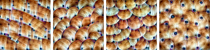
For example, let’s examine this simple optimization result.
 Simple optimization
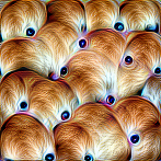
Looking at it in isolation one might infer that this neuron activates on the top of dog heads, as the optimization shows both eyes and only downward curved edges.
Looking at the optimization with diversity however, we see optimization results which don’t include eyes, and also one which includes upward curved edges. We thus have to broaden our expectation of what this neuron activates on to be mostly about the fur texture. Checking this hypothesis against dataset examples shows that is broadly correct. Note the spoon with a texture and color similar enough to dog fur for the neuron to activate.
Simple optimization
Looking at it in isolation one might infer that this neuron activates on the top of dog heads, as the optimization shows both eyes and only downward curved edges.
Looking at the optimization with diversity however, we see optimization results which don’t include eyes, and also one which includes upward curved edges. We thus have to broaden our expectation of what this neuron activates on to be mostly about the fur texture. Checking this hypothesis against dataset examples shows that is broadly correct. Note the spoon with a texture and color similar enough to dog fur for the neuron to activate.

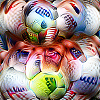
The effect of diversity can be even more striking in higher level neurons, where it can show us different types of objects that stimulate a neuron. For example, one neuron responds to different kinds of balls, even though they have a variety of appearances.


This simpler approach has a number of shortcomings:
For one, the pressure to make examples different can cause unrelated artifacts (such as eyes) to appear.
Additionally, the optimization may make examples be different in an unnatural way.
For example, in the above example one might want to see examples of soccer balls clearly separated from other types of balls like golf or tennis balls.
Dataset based approaches such as Wei et al.
Diversity also starts to brush on a more fundamental issue: while the examples above represent a mostly coherent idea, there are also neurons that represent strange mixtures of ideas. Below, a neuron responds to two types of animal faces, and also to car bodies.
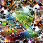


Examples like these suggest that neurons are not necessarily the right semantic units for understanding neural nets.
Interaction between Neurons
If neurons are not the right way to understand neural nets, what is? In real life, combinations of neurons work together to represent images in neural networks. A helpful way to think about these combinations is geometrically: let’s define activation space to be all possible combinations of neuron activations. We can then think of individual neuron activations as the basis vectors of this activation space. Conversely, a combination of neuron activations is then just a vector in this space.
This framing unifies the concepts “neurons” and “combinations of neurons” as “vectors in activation space”. It allows us to ask: Should we expect the directions of the basis vectors to be any more interpretable than the directions of other vectors in this space?
Szegedy et al.
Dataset examples and optimized examples of random directions in activation space. The directions shown here were hand-picked for interpretability.
We can also define interesting directions in activation space by doing arithmetic on neurons. For example, if we add a “black and white” neuron to a “mosaic” neuron, we obtain a black and white version of the mosaic. This is reminiscent of semantic arithmetic of word embeddings as seen in Word2Vec or generative models’ latent spaces.
By jointly optimizing two neurons we can get a sense of how they interact.
These examples show us how neurons jointly represent images.
To better understand how neurons interact, we can also interpolate between them.
This is only starting to scratch the surface of how neurons interact. The truth is that we have almost no clue how to select meaningful directions, or whether there even exist particularly meaningful directions. Independent of finding directions, there are also questions on how directions interact — for example, interpolation can show us how a small number of directions interact, but in reality there are hundreds of directions interacting.
The Enemy of Feature Visualization
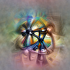
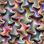
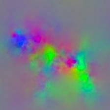
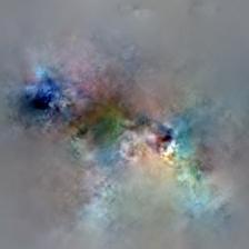
If you want to visualize features, you might just optimize an image to make neurons fire. Unfortunately, this doesn’t really work. Instead, you end up with a kind of neural network optical illusion — an image full of noise and nonsensical high-frequency patterns that the network responds strongly to.
Even if you carefully tune learning rate, you’ll get noise.
Optimization results are enlarged to show detail and artifacts.
These patterns seem to be the images kind of cheating, finding ways to activate neurons that don’t occur in real life.
If you optimize long enough, you’ll tend to see some of what the neuron genuinely detects as well,
but the image is dominated by these high frequency patterns.
These patterns seem to be closely related to the phenomenon of adversarial examples
We don’t fully understand why these high frequency patterns form,
but an important part seems to be strided convolutions and pooling operations, which create high-frequency patterns in the gradient
These high-frequency patterns show us that, while optimization based visualization’s freedom from constraints is appealing, it’s a double-edged sword. Without any constraints on images, we end up with adversarial examples. These are certainly interesting, but if we want to understand how these models work in real life, we need to somehow move past them…
The Spectrum of Regularization
Dealing with this high frequency noise has been one of the primary challenges and overarching threads of feature visualization research. If you want to get useful visualizations, you need to impose a more natural structure using some kind of prior, regularizer, or constraint.
In fact, if you look at most notable papers on feature visualization, one of their main points will usually be an approach to regularization. Researchers have tried a lot of different things!
We can think of all of these approaches as living on a spectrum, based on how strongly they regularize the model. On one extreme, if we don’t regularize at all, we end up with adversarial examples. On the opposite end, we search over examples in our dataset and run into all the limitations we discussed earlier. In the middle we have three main families of regularization options.
Frequency
Penalization
Transformation
Robustness
Learned
Prior
Dataset
Examples
Erhan, et al., 2009
Introduced core idea. Minimal regularization.
Szegedy, et al., 2013
Adversarial examples. Visualizes with dataset examples.
Mahendran & Vedaldi, 2015
Introduces total variation regularizer. Reconstructs input from representation.
Nguyen, et al., 2015
Explores counterexamples. Introduces image blurring.
Mordvintsev, et al., 2015
Introduced jitter & multi-scale. Explored GMM priors for classes.
Øygard, et al., 2015
Introduces gradient blurring.
(Also uses jitter.)
Tyka, et al., 2016
Regularizes with bilateral filters.
(Also uses jitter.)
Mordvintsev, et al., 2016
Normalizes gradient frequencies.
(Also uses jitter.)
Nguyen, et al., 2016
Paramaterizes images with GAN generator.
Nguyen, et al., 2016
Uses denoising autoencoder prior to make a generative model.
Three Families of Regularization
Let’s consider these three intermediate categories of regularization in more depth.
Frequency penalization directly targets the high frequency noise these methods suffer from.
It may explicitly penalize variance between neighboring pixels (total variation)
(Some work uses similar techniques to reduce high frequencies in the gradient before they accumulate in the visualization
Frequency penalization directly targets high frequency noise
Transformation robustness tries to find examples that still activate the optimization target highly even if we slightly transform them.
Even a small amount seems to be very effective in the case of images
Stochastically transforming the image before applying the optimization step suppresses noise
Learned priors. Our previous regularizers use very simple heuristics to keep examples reasonable. A natural next step is to actually learn a model of the real data and try to enforce that. With a strong model, this becomes similar to searching over the dataset. This approach produces the most photorealistic visualizations, but it may be unclear what came from the model being visualized and what came from the prior.
One approach is to learn a generator that maps points in a latent space to examples of your data,
such as a GAN or VAE,
and optimize within that latent space
Preconditioning and Parameterization
In the previous section, we saw a few methods
Transforming the gradient like this is actually quite a powerful tool — it’s called “preconditioning” in optimization.
You can think of it as doing steepest descent to optimize the same objective,
but in another parameterization of the space or under a different notion of distance.
How can we choose a preconditioner that will give us these benefits?
A good first guess is one that makes your data decorrelated and whitened.
In the case of images this means doing gradient descent in the Fourier basis,
 Correlated Colors
 Decorrelated Colors
Let’s see how using different measures of distance changes the direction of steepest descent. The regular L2 gradient can be quite different from the directions of steepest descent in the L∞ metric or in the decorrelated space:
All of these directions are valid descent directions for the same objective, but we can see they’re radically different. Notice that optimizing in the decorrelated space reduces high frequencies, while using L∞ increases them.
Using the decorrelated descent direction results in quite different visualizations. It’s hard to do really fair comparisons because of hyperparameters, but the resulting visualizations seem a lot better — and develop faster, too.
Combining the preconditioning and transformation robustness improves quality even further
(Unless otherwise noted, the images in this article were optimizing in the decorrelated space and a suite of transformation robustness techniques.
• Padding the input by 16 pixels to avoid edge artifacts
• Jittering by up to 16 pixels
• Scaling by a factor randomly selected from this list: 1, 0.975, 1.025, 0.95, 1.05
• Rotating by an angle randomly selected from this list; in degrees: -5, -4, -3, -2, -1, 0, 1, 2, 3, 4, 5
• Jittering a second time by up to 8 pixels
• Cropping the padding
Is the preconditioner merely accelerating descent, bringing us to the same place normal gradient descent would have brought us if we were patient enough? Or is it also regularizing, changing which local minima we get attracted to? It’s hard to tell for sure. On the one hand, gradient descent seems to continue improving as you exponentially increase the number of optimization steps — it hasn’t converged, it’s just moving very slowly. On the other hand, if you turn off all other regularizers, the preconditioner seems to reduce high-frequency patterns.
Conclusion
Neural feature visualization has made great progress over the last few years. As a community, we’ve developed principled ways to create compelling visualizations. We’ve mapped out a number of important challenges and found ways of addressing them.
In the quest to make neural networks interpretable, feature visualization stands out as one of the most promising and developed research directions. By itself, feature visualization will never give a completely satisfactory understanding. We see it as one of the fundamental building blocks that, combined with additional tools, will empower humans to understand these systems.
There remains still a lot of important work to be done in improving feature visualization. Some issues that stand out include understanding neuron interaction, finding which units are most meaningful for understanding neural net activations, and giving a holistic view of the facets of a feature.